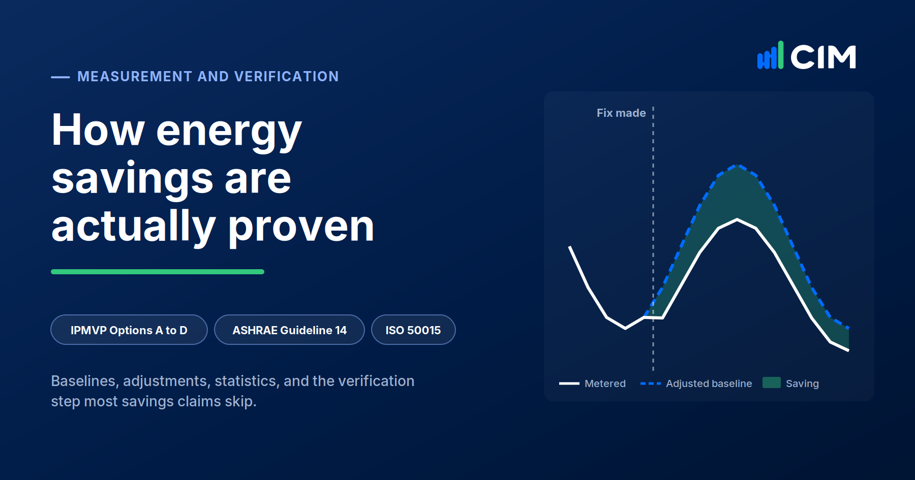
Every building analytics vendor, energy service company and commissioning firm claims savings. Very few of those claims survive a simple question: compared with what?
A saving is energy that was not used. You cannot put a meter on it. The only way to prove one is to establish, credibly, how much energy the building would have used without the change, and compare that with what it actually used. That process has a name, measurement and verification, and an established body of method behind it: the International Performance Measurement and Verification Protocol (IPMVP), ASHRAE Guideline 14, the US federal FEMP guidelines and ISO 50015.
This guide explains how that method works in commercial buildings, where it breaks, and the step most savings claims skip entirely: confirming that the fix behind the saving actually happened, and stayed fixed.
In practice, an honest savings claim has to answer three questions, not one. Was the fault actually fixed? Did it stay fixed? Did energy actually fall? Conventional M&V answers only the third, usually once a year. The sections below cover the methodology for that third question in full, then show how the first two close the gap.
Key takeaways
- Savings cannot be measured directly. They are calculated as the gap between an adjusted baseline and metered consumption.
- IPMVP defines four options. A and B isolate a single measure, C measures the whole facility, D uses a calibrated simulation.
- Adjustments decide whether the number is honest. Routine adjustments handle weather and occupancy. Non-routine adjustments handle one-off changes, and an unlogged one can quietly inflate or erase a reported saving.
- ASHRAE Guideline 14 supplies the statistics. CV(RMSE) and NMBE tell you whether a baseline model is good enough to rely on.
- Meter-level M&V cannot tell you which fix worked. Proving a saving also means proving each fault was fixed and stayed fixed.
What is measurement and verification?
Measurement and verification (M&V) is the process of using measurement to reliably determine the energy, demand or water savings delivered by a project or energy conservation measure (ECM). It estimates what the building would have consumed had the project not happened, adjusts that estimate for anything else that changed, and compares it with what the meters recorded.
M&V grew up around energy performance contracts, where an energy service company is paid from the savings it delivers and both sides need a number they can agree on. It is now used far more widely: utility incentive programmes paying per verified kilowatt-hour, green leases, sustainability-linked finance, internal business cases, and any board asking whether last year's efficiency spend worked. We covered how that pressure is reshaping the ESCO model in how analytics software supports energy service companies.
M&V is distinct from three things it is often confused with. Energy monitoring tells you what a building used. Energy benchmarking compares that use against similar buildings, as described in our guide to energy benchmarking. Fault detection tells you what is wrong. None of them, on its own, tells you how much a specific intervention saved.
How are energy savings calculated?
Energy savings are calculated as baseline energy minus reporting-period energy, plus or minus routine and non-routine adjustments. Every IPMVP-adherent savings calculation reduces to this one equation:
Savings = (Baseline energy - Reporting-period energy) ± Routine adjustments ± Non-routine adjustments
The baseline period is a stretch of time before the change, used to learn how the building uses energy. The reporting period is the time after the change, over which savings are claimed. The adjustments restate the baseline under reporting-period conditions, so that the comparison is like for like.
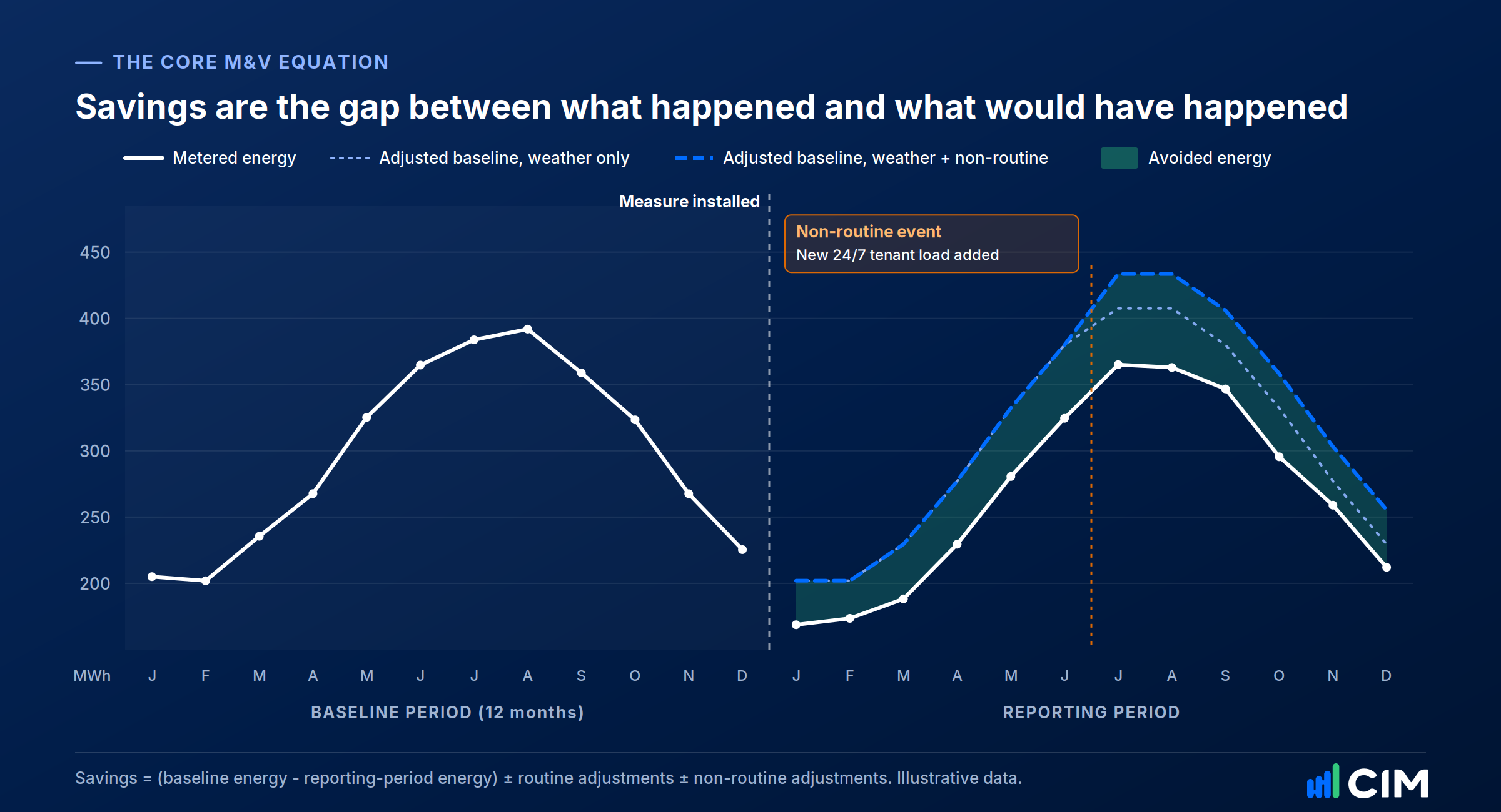
Without adjustment, the comparison is meaningless. A mild summer will make a failed project look like a success. A new tenant running servers around the clock will make a successful one look like a failure. The chart above shows both at work: the adjusted baseline rises with a hotter reporting year, and steps up again when a non-routine load is added, so the saving is measured against the building as it now is.
Avoided energy use versus normalised savings
IPMVP recognises two ways of stating the result, and mixing them up causes more disputes than any statistical error.
| Avoided energy use | Normalised savings | |
|---|---|---|
| Question answered | What would the building have used this year without the measure? | What does the measure save under a typical, fixed set of conditions? |
| Conditions used | The actual conditions of the reporting period | A fixed set, often a typical weather year |
| Models needed | A baseline model only | A baseline model and a reporting-period model |
| Best for | Contract payments and incentive claims for a specific period | Year-on-year comparison and long-term planning |
| Watch out for | Results swing with an extreme year even when the measure performs steadily | More modelling error, because two models contribute uncertainty |
EVO's own guidance notes that normalised savings carry more modelling error than avoided energy use, because a second model is being fitted and adjusted (EVO, Advanced M&V white paper). Agree which one you are reporting before the reporting period starts.
What are the four IPMVP options?
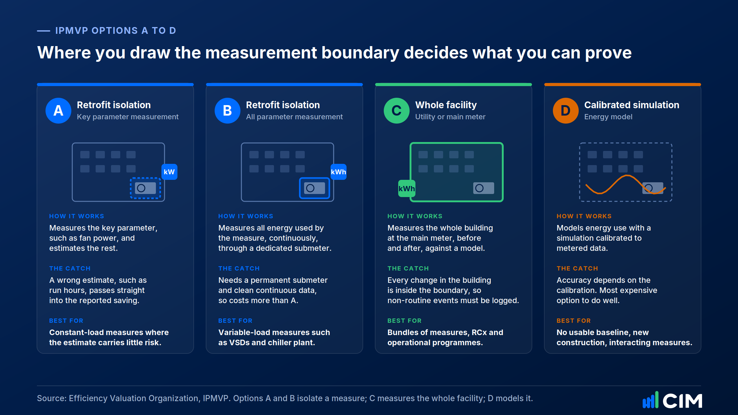
IPMVP defines four ways to determine savings. Options A and B isolate a single measure, measuring either its key parameter (A) or all of its energy use (B). Option C measures the whole facility at the main meter. Option D uses a computer simulation calibrated to metered data, typically where no usable baseline exists.
IPMVP is maintained by the Efficiency Valuation Organization. It is deliberately a framework rather than a rulebook, and its most important structural decision is the measurement boundary: the line drawn around whatever is being measured. Draw it around a single fan and you can prove what that fan saved. Draw it around the whole building and you capture every interaction, along with everything else that changed.
| Option | What is measured | What can be estimated | Typical building applications |
|---|---|---|---|
| A: Retrofit isolation, key parameter | The parameter that defines the saving, such as fan power | Other parameters, such as operating hours, if justified and agreed | Lighting retrofits, constant-speed motor replacements, fixed schedule corrections |
| B: Retrofit isolation, all parameters | All energy used by the measure, continuously | Nothing material | Variable speed drives, chiller plant optimisation, pump and fan control strategies |
| C: Whole facility | The main utility or sub-meter, before and after | Nothing, but every change inside the boundary must be adjusted for | Retro-commissioning, bundles of operational measures, whole-building programmes |
| D: Calibrated simulation | Enough metered data to calibrate a model | The baseline itself, which is simulated | New construction, major refurbishment, projects with no usable baseline |
Two things are worth saying plainly about these options, because they are often glossed over.
Option A is only as good as its estimate. If a variable speed drive is proven by measuring power once and assuming run hours, and the run hours were wrong, the reported saving is wrong by the same proportion. That is acceptable when the estimated parameter is stable and genuinely outside anyone's control. It is not acceptable when the estimate is the thing most likely to change, which, in commercial HVAC, run hours usually are.
Option C sees everything, including things you did not do. The main meter cannot tell a retro-commissioning saving from a tenant who moved out. Option C works when the saving is large enough to stand out from normal variation, and when somebody is keeping a disciplined log of every other change inside the boundary. At one London headquarters, for example, a 14% year-on-year fall at the main meter stood out clearly against a pre-existing trend of around 3%, as described in how a London headquarters cut electricity use by 14% in 11 weeks.
How do you choose an IPMVP option?
Choose by asking three questions: can energy be measured before the change, is the saving large enough to see at the main meter, and can one measured parameter define it? Those three questions narrow most projects to a single option.
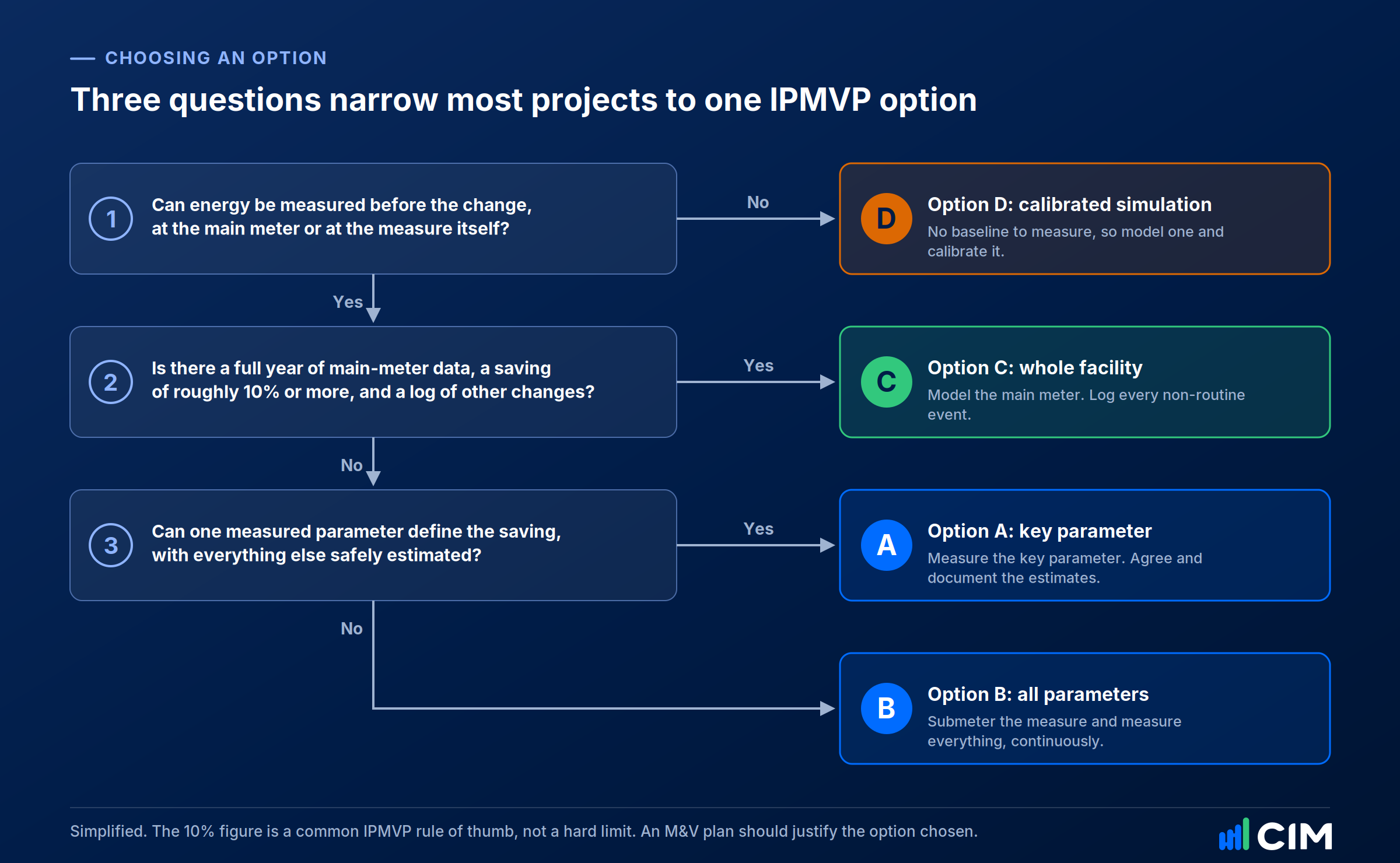
The threshold in question two deserves explanation. IPMVP's own rule of thumb is that where only monthly billing data are available, savings typically need to exceed around 10% of baseline energy to be distinguished from unexplained variation. It is a rule of thumb tied to monthly data, not a limit. An EVO paper on ComEd's virtual commissioning programme describes whole-building analysis on interval data identifying savings as low as 3% of facility consumption. With noisy monthly bills, by contrast, even 10% can disappear into the error.
This matters for fault-driven programmes. Correcting a single passing valve can be worth tens of thousands a year and still be a small fraction of a large tower's total consumption. In our analysis of the most common HVAC faults across 600+ buildings, the largest verified single-fault savings came from individual air handling units. Proving savings like those at the main meter is hard. Proving them at the equipment boundary, with Option A or B, is far more reliable.
How do you build an M&V baseline?
A sound M&V baseline covers a full operating cycle, usually twelve months. It models energy against the variables that drive it, such as weather and occupancy, documents the static factors assumed not to change, and is built on data that can be trusted. Each of those four decisions can quietly break it.
The baseline period. It should cover a full operating cycle, which for most commercial buildings means twelve months so that every season is represented. It should also be representative: a baseline that includes months of plant running in override, or a floor sitting empty, bakes that condition into every future saving.
The independent variables. These are the factors expected to change and drive energy use: outside air temperature or degree days, occupancy, operating hours, and for some buildings production or visitor numbers. Each must be measured over the same intervals as the energy data. Plotting consumption against weather before fitting anything is the fastest sanity check available, and it is exactly what PEAK's weather comparison charts were built for.
The static factors. These are the conditions assumed not to change: floor area, building use, installed equipment, hours of operation as contracted. They must be documented at the start, because any later change to them becomes a non-routine adjustment, and you cannot adjust for a change to something you never recorded.
The data itself. A baseline model is only as trustworthy as the meters and sensors behind it. Gaps have to be handled transparently. PEAK's meter gap filling, for example, estimates missing electricity data from the same weekday over the previous four weeks and replaces estimates automatically when actual data arrives. Whatever method is used, the M&V plan should state it. And the underlying points need to mean what they say, which is a data layer problem we covered in BMS point naming, Haystack and Brick.
That last point is not theoretical. At one site, a contractor replaced a pressure sensor with one of a different range and the BMS was never reconfigured. The BMS reported 12,782 m³/h of airflow while an independent instrument measured 32,460 m³/h, and the fan ran at 100% for months. The case is written up in holding contractors accountable: how PEAK uncovered a costly oversight. Any baseline or savings calculation built on that sensor would have been wrong from the first day.
What are routine and non-routine adjustments?
Routine adjustments correct the baseline for factors expected to change, such as weather and occupancy, through the baseline model. Non-routine adjustments correct it for one-off changes to the building, such as added floor area or a new tenant load, case by case. Together they separate a defensible saving from a convenient one.
| Routine adjustments | Non-routine adjustments | |
|---|---|---|
| What they account for | Factors expected to change and affect energy use | One-off changes to the static factors |
| Examples | Weather, occupancy levels, operating hours | Added floor area, a new 24/7 tenant load, a data room, equipment added or removed, a change of building use |
| How they are made | Automatically, through the baseline model | Case by case, by engineering calculation or a separate model |
| What goes wrong | A poorly fitted model under-adjusts or over-adjusts every period | The event is never logged, so the saving silently absorbs it |
EVO describes non-routine events as a key risk for any project using meter-based M&V, and published a dedicated IPMVP application guide on non-routine events and adjustments in 2020. Unaccounted events, it notes, can introduce unacceptable levels of error, and the risk matters most wherever M&V is the basis for payment. The guide was released during the COVID-19 pandemic, which EVO itself described as one of the most far-reaching non-routine events of recent times.
Not every non-routine event is a new tenant. Some are operational. After an annual fire test at one retail site, several systems were left in manual override and plant began running overnight. Detected in real time, it was corrected within a day. Left for a quarter, it would have added an estimated 8% to the site's energy use, as described in real-time anomaly detection prevents 8% energy drift. In an Option C calculation, an event like that either erodes a genuine saving or, if someone later tidies the data, disappears without trace.
What does ASHRAE Guideline 14 require?
ASHRAE Guideline 14 sets the statistical tests a baseline model or calibrated simulation must pass before savings calculated from it are relied on. The core metrics are CV(RMSE), which measures scatter, and NMBE, which measures bias.
IPMVP tells you what to do. Guideline 14 tells you whether you did it well enough. It is intended for transactions where savings are the basis for payment, and it sets out calculation procedures and the minimum statistical performance a baseline model or calibrated simulation should achieve. The 2023 edition expands the treatment of uncertainty and adds sections on cost estimation, the ASHRAE Inverse Modeling Toolkit and long-term data storage. A 2024 errata sheet set the limit on net determination bias for regression models at 0.5%, and a 2025 addendum retitled the guideline Measurement and Verification of Energy, Demand, and Water Savings.
| Metric | What it tells you | Commonly applied threshold | Where it applies |
|---|---|---|---|
| CV(RMSE), coefficient of variation of the root mean square error | How closely the model tracks each individual data point | 15% or less on monthly data, 30% or less on hourly data | Calibrated simulation (Option D) |
| NMBE, normalised mean bias error | Whether the model consistently over-predicts or under-predicts | Within ±5% on monthly data, ±10% on hourly data | Calibrated simulation (Option D) |
| Net determination bias of a regression model | How much the model's total prediction differs from the total measured over the baseline period | 0.5% or less, per the 2024 errata | Regression baselines, whole-building and retrofit isolation |
| CV(RMSE) of a baseline regression | How much scatter remains after the model explains weather and other variables | 25% or less with 12 to 60 months of data | Whole-building baselines (Option C) |
| Fractional savings uncertainty | How large the uncertainty is relative to the saving being claimed | Often specified as less than 50% at 68% confidence | Programme and contract acceptance criteria |
The calibration thresholds are widely reproduced in the research literature (for example, this Oak Ridge validation paper). Utility programmes and contracts frequently add their own criteria on top. One Texas programme filing, for instance, requires an NMBE below 0.5%, a CV(RMSE) below 25% and savings uncertainty below 50% at 68% confidence. Check the criteria in your own contract or programme rules, because they override the guideline defaults.
The practical lesson is that model fit is not a formality. Stricter acceptance criteria can actually increase verified savings, because a tighter model lets smaller savings be distinguished from noise rather than written off as within the error.
How do IPMVP, Guideline 14, FEMP and ISO 50015 differ?
IPMVP is the framework, ASHRAE Guideline 14 supplies the statistics, the FEMP guidelines apply IPMVP to US federal performance contracts, and ISO 50015 sets principles for organisation-level M&V. They overlap, and they are often cited as though they were interchangeable. They are not.
| Document | Published by | What it is for | Where you meet it |
|---|---|---|---|
| IPMVP Core Concepts (2022) | Efficiency Valuation Organization | The framework: savings equation, Options A to D, M&V plan contents | Energy performance contracts worldwide, utility programmes, green finance |
| ASHRAE Guideline 14-2023 | ASHRAE | Calculation procedures and statistical acceptance criteria | US contracts and programmes, and as the statistical reference behind many others |
| FEMP M&V Guidelines 5.0 (2024) | US Department of Energy | Application of IPMVP to federal performance contracts, with guidance for specific measures | US federal ESPCs and many state programmes that borrow from them |
| ISO 50015 | ISO | Principles for measuring and verifying the energy performance of an organisation | Organisations running an ISO 50001 energy management system |
| ISO 50006 | ISO | Energy baselines and energy performance indicators | ISO 50001 programmes tracking performance over time |
| ISO 17741 | ISO | General rules for measuring, calculating and verifying project savings | International project-level savings, often alongside IPMVP |
The US federal guidance is a useful practical reference even outside the US. FEMP's M&V Guidelines Version 5.0, released in October 2024, updated the 2015 edition with clarification on applying the IPMVP options and expanded guidance for specific energy conservation measures. In Australia, schemes such as the NSW Energy Savings Scheme include measurement and verification methods of their own, grounded in the same IPMVP concepts.
What is advanced M&V (M&V 2.0)?
Advanced M&V, often called M&V 2.0, uses interval meter data and automated baseline models to calculate savings continuously, rather than once a year from monthly bills.
Traditional M&V fitted a regression to twelve monthly utility bills and reported once a year. With 15-minute interval data and modern modelling, that is no longer the only option.
The evidence that it works is solid. Lawrence Berkeley National Laboratory tested ten automated baseline models against 15-minute meter data from 537 commercial buildings. With twelve months of training data, median CV(RMSE) was under 25% for every model tested. With just six months, median CV(RMSE) on daily totals was still under 25% for all models (Granderson et al., 2016).
Open methods have followed. The CalTRACK methods, developed through an open stakeholder process, standardise how metered savings are calculated from monthly, daily and hourly data. Their reference implementation, the open-source OpenEEmeter library, has since been extended as OpenDSM under LF Energy. For anyone buying or specifying advanced M&V, the practical test is the same: can the vendor show the model, its fit statistics and its data rules, rather than a savings number alone?
The operational consequence matters more than the statistics. Continuous baselines mean a saving can be tracked as it emerges rather than discovered a year later, and an erosion can be spotted in weeks rather than at the annual reconciliation. That is the same shift that turned commissioning from a one-off project into monitoring-based commissioning. Within PEAK's energy management capability, the energy performance dashboard tracks consumption against targets and baselines on this basis.
Why do verified savings decay?
Verified savings decay because many of them come from operational changes, such as schedules, setpoints and control sequences, that are easily undone. The research on persistence is consistent in direction, if not in exact numbers.
A Slipstream review of retro-commissioning persistence found average savings persistence of 76% across the studies it examined, covering one to eight years after the work. A ComEd programme study suggested degradation happens mostly in the first few years after RCx rather than steadily, and found one measure, optimum start for air handling units, with zero persistence across the instances observed. A long-running Texas A&M study of ten university buildings tracked the same decline year by year.
The pattern behind the numbers is familiar to anyone who has run a retro-commissioning project. Hardware changes persist. Operational changes, the schedules, setpoints, resets and control sequences that deliver most RCx savings, get undone. A callout puts a unit in hand. A complaint drops a setpoint. A sensor drifts and takes a reset strategy with it.
This is also why fault detection programmes deliver less than their potential. Correcting common building faults is estimated to be worth 5 to 30% of whole-building energy, but organisations in the US Department of Energy's Smart Energy Analytics Campaign reported a median of 9%. The gap is not detection. It is faults that were found and never fixed, or fixed and never kept fixed.
The verification gap: why meter-level M&V is not enough
Meter-level M&V can prove that energy fell. It cannot prove which fixes delivered, which failed, and which were never carried out. A retro-commissioning programme of thirty findings can report a healthy Option C saving while five of those findings were closed on a contractor's word and never actually done.
Honest savings verification has to answer three questions, not one.
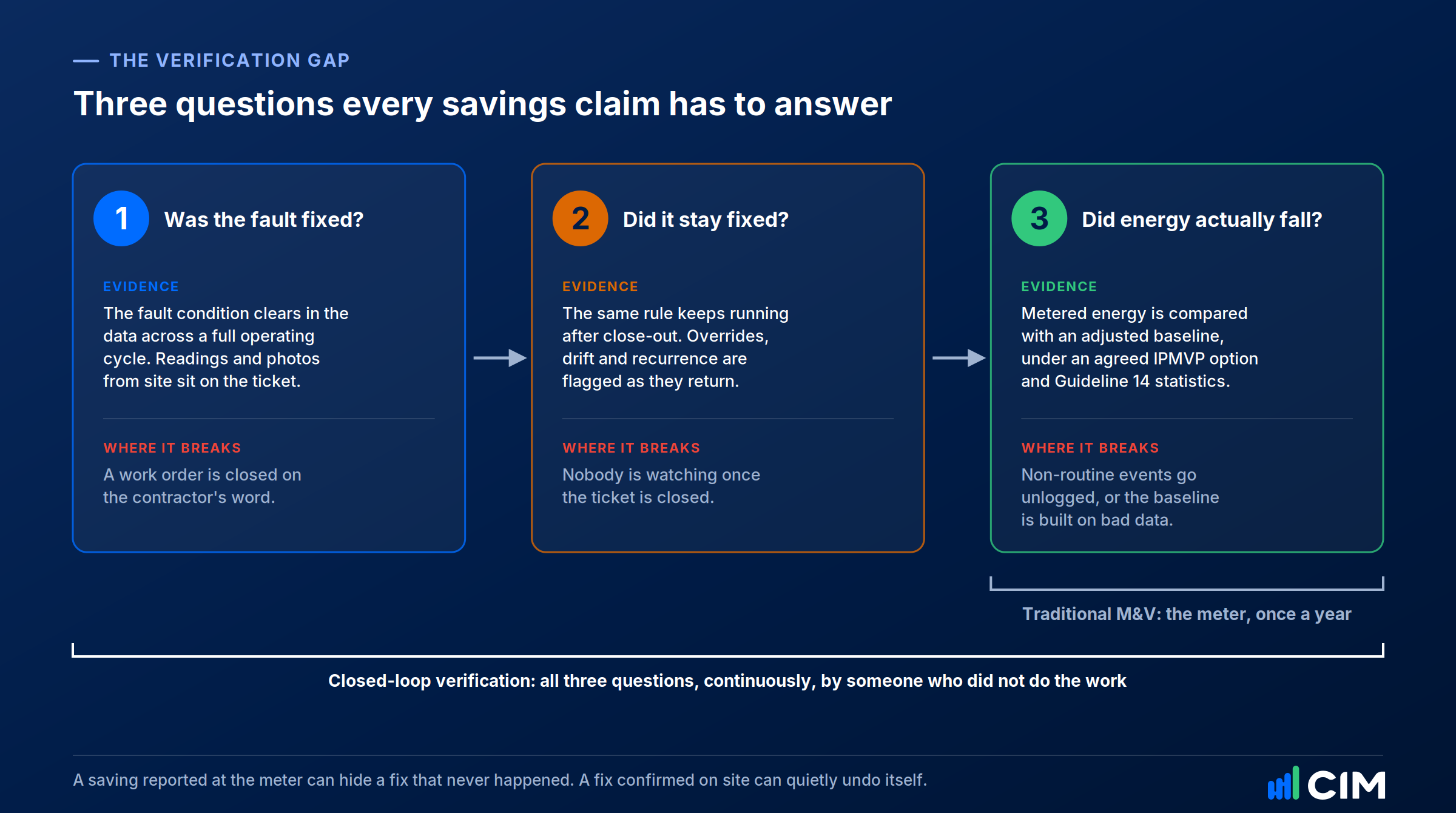
1. Was the fault actually fixed? The evidence is the fault condition clearing in the data across a full operating cycle, backed by readings from site. At one London tower, engineers took a live chilled water valve alert to the plant room, measured a 6.1 VDC control signal at the actuator, found the valve stem 40% open against a 0% command, and had the evidence on the ticket 98 minutes after the session began, as told in sceptical engineers confirm a £25,000 fault in 98 minutes. That is field verification of the fault. The estimated saving attached to it only becomes a verified saving once the valve is rectified and the result is measured.
2. Did it stay fixed? The same rule that raised the fault keeps running after close-out, so an override that returns, a schedule that creeps back, or a sensor that drifts again is flagged as it happens. This is the question that the persistence research says matters most, and the one no annual M&V report can answer in time to do anything about it.
3. Did energy actually fall? This is classic M&V: metered consumption against an adjusted baseline under an agreed IPMVP option, tested with Guideline 14 statistics. It remains essential, because it is the only question whose answer carries contractual weight.
The third question without the first two produces numbers nobody can explain. The first two without the third produce activity nobody can value. And all three need to be answered by someone other than the party whose work is being measured. Nobody should be marking their own homework, which is the principle behind independent building monitoring.
Where PEAK fits in an M&V process
PEAK is not a substitute for an M&V plan agreed between the parties to a contract, and does not claim to be. What it supplies is the evidence an M&V process depends on and usually lacks.
- Fault-level verification. Through PEAK's fault detection and diagnostics, each fault is tracked from detection through a named owner to closure, with the rule confirming it has cleared and continuing to watch for recurrence. This answers questions one and two continuously.
- Clean, continuous data. BMS-agnostic integration across mixed estates, normalised point data, and transparent handling of meter gaps give baseline models something trustworthy to be built on.
- A log of non-routine events. Overrides, out-of-hours operation and equipment changes are surfaced as they occur, which is exactly the record Option C depends on.
- Honest labelling of estimates. PEAK's automated cost savings estimate the financial impact of energy faults so they can be prioritised. They are estimates for triage, not verified savings, and should be treated that way in any M&V report.
What should an M&V plan include?
IPMVP describes the contents of an M&V plan in detail. At a minimum, a plan that will survive a dispute records:
- The intent of each measure and the savings expected from it
- The IPMVP option selected and the measurement boundary
- The baseline period, its energy data and the conditions that applied
- The static factors, documented well enough to detect a later change
- The reporting period and how often savings will be reported
- The basis for routine adjustments and how non-routine events will be identified and handled
- The analysis method, including how data gaps are treated
- The energy prices used to value savings
- Meter specifications, calibration and who is responsible for monitoring
- The expected accuracy, and the acceptance criteria any model must meet
- The report format and the quality assurance process
What this means for engineering partners
For retro-commissioning firms, MBCx providers, ESCOs and controls contractors, M&V is not paperwork. It is the mechanism by which work gets paid for, renewed and referred.
Utility programmes commonly pay incentives on verified savings. Performance contracts pay from them. Clients renew monitoring retainers when a quarterly report shows verified outcomes rather than activity. Aero Performance Group, a leading RCx and MBCx provider in its utility programme, now verifies around 6 million kWh of energy-saving incentives a year for its clients, and its commissioning manager talks through how fault data changed that delivery in our webinar on how FDD improves RCx and MBCx outcomes.
Three practical implications follow. Choose the IPMVP option at the proposal stage, not after the work is done. Log non-routine events from day one, because reconstructing them later is where disputes start. And separate the evidence that a fault was fixed from the calculation of what fixing it saved, because clients increasingly want both. Where independent M&V is required, the recognised credential is the Certified Measurement and Verification Professional (CMVP), which is also an approved credential under Boston's BERDO ordinance. Our guides to running RCx and MBCx on fault detection and costing remedial works from FDD cover the delivery side in more depth.
Prove the fix, then prove the saving
The Building Performance Engineer's FDD Playbook covers the closed loop from detection to verified rectification, and how verified outcomes turn projects into recurring revenue.
Download the playbookTalk to our partner teamFrequently asked questions
What is measurement and verification (M&V)?
Measurement and verification is the process of using measurement to reliably determine the energy, demand or water savings a project actually delivered. Because a saving is the absence of energy use, it cannot be metered directly. M&V estimates what the building would have used without the change, adjusts that estimate for conditions such as weather, and compares it with what was actually metered.
What is IPMVP?
IPMVP, the International Performance Measurement and Verification Protocol, is the most widely used framework for determining energy savings. It is maintained by the Efficiency Valuation Organization (EVO). It defines the savings equation, the four measurement options A to D, and the contents of an M&V plan. It is a framework rather than a prescriptive standard, so each project documents how it applies it.
Which IPMVP option suits retro-commissioning and operational fixes?
Option C is the usual choice when a programme bundles many small operational measures and the combined saving is large relative to whole-building consumption. When the saving is small against the main meter, or a single measure needs to be proven on its own, Option A or B at the equipment level is more reliable, provided the key parameters can be measured.
Can you verify the saving from a single fault fix?
Usually not at the main meter, because a single fix is often too small relative to whole-building consumption to separate from normal variation. It can be verified at the equipment level using IPMVP Option A or B: confirm the fault condition has cleared across a full operating cycle, then measure, or reliably estimate, the energy use of the affected plant before and after the fix.
Can energy savings be verified using BMS data instead of utility meters?
Partly. BMS trend data such as run hours, fan speed, valve position and plant power can support Option A or B verification at the equipment level, and can document non-routine events as they happen. It is only as reliable as the sensors behind it, so critical points should be checked against independent measurement, and most contracts still settle on utility or calibrated sub-meter data.
What is ASHRAE Guideline 14?
ASHRAE Guideline 14 is a technical guideline for measuring energy, demand and water savings. It sets out calculation procedures and the statistical tests a baseline model or calibrated simulation should pass before savings calculated from it are relied on. The current edition is Guideline 14-2023, amended by a 2024 errata sheet and a 2025 addendum.
How long should an M&V baseline period be?
Long enough to cover a full operating cycle, which for most commercial buildings means 12 months so that every season is represented. Shorter baselines can work with interval meter data: Lawrence Berkeley National Laboratory testing found several automated models still performed acceptably on daily totals with six months of training data.
Is IPMVP the same as ISO 50015 or ASHRAE Guideline 14?
No. IPMVP is the conceptual framework for determining savings. ASHRAE Guideline 14 adds technical procedures and statistical acceptance criteria. ISO 50015 sets out principles for measuring and verifying the energy performance of an organisation, and references IPMVP. In practice, a project often follows IPMVP for its structure and Guideline 14 for its statistics.
Is M&V required for utility incentives or energy performance contracts?
Generally, yes. Energy performance contracts pay from verified savings, so the contract defines an M&V plan, usually based on IPMVP. Utility programmes that pay incentives on measured savings typically specify an M&V method and model acceptance criteria as well. The exact requirements are set by the contract or programme rules, which take precedence over guideline defaults.
What is a CMVP?
A CMVP is a Certified Measurement and Verification Professional, a credential awarded by the Association of Energy Engineers and offered in conjunction with EVO. It requires passing an exam and meeting academic and practical experience requirements. It is recognised in several programmes, including as an approved credential under Boston's BERDO 2.0 ordinance.
Why do verified savings decline over time?
Because many savings come from operational changes that can be undone. Schedules are extended, points are overridden, setpoints are changed after a complaint and sensors drift. A Slipstream review of retro-commissioning studies found average savings persistence of 76%, and controls-based measures are typically the least durable. Continuous monitoring is what catches the reversal.
Does fault detection software replace M&V?
No. Fault detection confirms that individual faults were fixed and stay fixed, which is evidence an M&V process needs but does not produce on its own. M&V quantifies the energy saving at the meter against an adjusted baseline, under a plan agreed by both parties. The two answer different questions and work best together.
Sources: Efficiency Valuation Organization, IPMVP Core Concepts and the IPMVP Application Guide on Non-Routine Events and Adjustments; ASHRAE Guideline 14-2023, with its 2024 errata sheet and 2025 addendum; US Department of Energy FEMP M&V Guidelines Version 5.0; Kelly and Sinnamon, EVO M&V Focus, 2020; Granderson et al., Applied Energy, 2016; LF Energy OpenDSM; Association of Energy Engineers; Slipstream; ComEd and Seventhwave; Texas A&M Energy Systems Laboratory; US DOE Smart Energy Analytics Campaign. Statistical thresholds are the commonly cited defaults. Contract and programme criteria take precedence.

A practical playbook for the engineers who deliver building performance. Learn how to run retro-commissioning, monitoring-based commissioning and data-driven maintenance on an FDD platform: compress the RCx cycle from 12-18 months to 3-5, close the loop from alert to verified fix, and turn fixed-term projects into recurring revenue. Written for RCx and MBCx firms, engineering consultancies, and BMS and mechanical contractors.
PEAK uncovered a contractor error, preventing energy waste and equipment failures.
Read the story →